Multi-view Geometry 0 Background
This is a learning note for the book: Multiple View Geometry in Computer Vision, Second Edition.
Projective Geometry and Transformations of 2D
Line and point
-
Definition (inhomogeneous $\Leftrightarrow$ homogeneous):
$$ax+by+c=0 \Leftrightarrow \mathbf{x}^\top\mathbf{L}=0$$
Degree of freedom (dof) = 2 -
Homogeneous form of Line:
$$\mathbf{L}=k(a,b,c)^\top \in \mathbb{R}^3$$ -
Homogeneous form of point:
$$\mathbf{x}=(x_1,x_2,x_3)^\top \in \mathbb{R}^3 \\
\Rightarrow (\frac{x_1}{x_3},\frac{x_1}{x_3})\in\mathbb{R}^2 $$ -
Intersection of lines:
$$\mathbf{x}=\mathbf{L}_1\times\mathbf{L}_2$$
Because in vector computation (triple scalar product, think in 3D space):
$$\mathbf{L}_1(\mathbf{L}_1\times\mathbf{L}_2)=\mathbf{L}_2(\mathbf{L}_1\times\mathbf{L}_2)\\
\Rightarrow \mathbf{L}_1\mathbf{v}=\mathbf{L}_2\mathbf{v}\\
\Rightarrow \mathbf{v}=\mathbf{x}$$ -
Line through two points:
$$\mathbf{L}=\mathbf{x}_1\times\mathbf{x}_2$$
Use the same trick above. -
Ideal points (the point two parallel line intersect on):
$$\mathbf{x}_{ideal}=(x_1,x_2,0)^\top\in\mathbb{R}^3$$ -
Line at infinity (The set of ideal points lies):
$$\mathbf{L}_\infty=(0,0,1)^\top\in\mathbb{R}^3$$ -
Projective Plane:
Points and lines of $\mathbb{P}^2$ are represented by rays and planes in $\mathbb{R}^3$ respectively. Ideal points are the vectors lying in $x_1x_2$-plane, and $\mathbf{L}_\infty$ is $x_1x_2$-plane.

-
Duality principle
In 2D projective geometry, any theorem has dual theorem by interchanging lines and points.
Conics
-
Definition (inhomogeneous $\Leftrightarrow$ homogeneous):
$$ax^2+bxy+cy^2+dx+ey+f=0 \\
\Leftrightarrow ax_1^2+bx_1x_2+cx_2^2+dx_1x_3+ex_2x_3+fx_3^2=0 \\
where, x\rightarrow \frac{x_1}{x_3},y\rightarrow \frac{x_2}{x_3}$$In matrix form:
$$\mathbf{x}^\top C \mathbf{x}=0 \\
where, C=\begin{bmatrix}
a & \frac{b}{2} & \frac{d}{2} \\
\frac{b}{2} & c & \frac{e}{2} \\
\frac{d}{2} & \frac{e}{2} & f
\end{bmatrix}$$Dof: 5 (The ratios $\{a:b:c:d:e:f\}$)
-
Tangent lines to conics:
$$\mathbf{L}=C\mathbf{x}$$ -
Line conic definition:
$$\mathbf{L}^\top C^* \mathbf{L}=0$$$$C^*=C^{-1}$$

Transformations
-
Projection transformation:
$$\mathbf{x}'=H\mathbf{x}, \mathbf{x}\in\mathbb{R}^3$$
, where $H$ is non-sigular matrix. -
Transformation of lines:
$$\mathbf{L}'=H^{-\top}\mathbf{L}$$ -
Transformation of conics:
When $\mathbf{x}‘=H\mathbf{x}$,
$$\mathbf{x}^\top C\mathbf{x}=[H^{-1}\mathbf{x}’]^\top C H^{-1}\mathbf{x}‘\\
=\mathbf{x}’^\top [H^{-\top}CH^{-1}]\mathbf{x}‘\\
=\mathbf{x}’^\top C’\mathbf{x}'$$
and for line conics,
$$C^{*\prime}=HC^*H^\top$$ -
Different transformations

$$R = \begin{bmatrix}
cos\theta & -sin\theta \\
sin\theta & cos\theta
\end{bmatrix}$$ -
The topology of the projective plane
Think about $\mathbb{P}^2$ and unit sphere in $\mathbb{R}^3$, there is a two-to-one correspoindence between the unit sphere $S^2 \in \mathbb{R}^3$ and projective plane $\mathbb{P}^2$. In the language of topology, the sphere $S^2$ is a 2-sheeted covering space of $\mathbb{P}^2$.
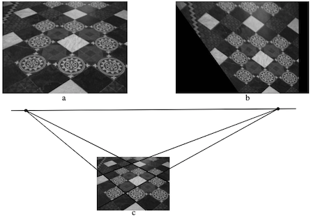
Recovery of affine and metric properties from images

- The line at infinity $\mathbf{L}_\infty$ is a fixed line the projective transformation $H$ if and only if $H$ is a afinity

-
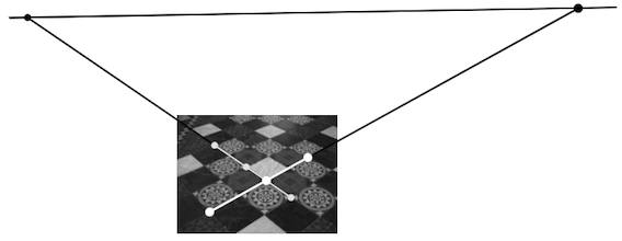
We can compute vanishing point from parallel line:
-
Also we can compute from a length ratio (see p.51 for more detail):
-
The circular points $\mathbf{I}, \mathbf{J}$ are fixed points under the projective transformation $H$ if and only if $H$ is a similarity (proof: p.52)
$$\mathbf{I}=(1, i, 0)^\top\\
\mathbf{J}=(1, -i, 0)^\top$$ -
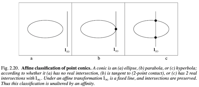
Classification of conics
Projective Geometry and Transformation of 3D
Points, Lines, and projective transformations
-
Points (homogeneous$\Leftrightarrow$inhomogeneous): $(X_1,X_2,X_3,X_4)^\top \Leftrightarrow (\frac{X_1}{X_4},\frac{X_2}{X_4},\frac{X_3}{X_4})^\top$
-
Planes (dof: 3):
$$\pi_1X+\pi_2Y+\pi_3Z+\pi_4=0\\
\Leftrightarrow \pi_1X_1+\pi_2X_2+\pi_3X_3+\pi_4X_4=0\\
\Leftrightarrow \boldsymbol{\pi}^\top\mathbf{X}=0$$ -
In $\mathbb{P}^3$, points and planes are dual and lines are self-dual.
-
Three points define a plane:
$$\begin{bmatrix}
\mathbf{X}_1^\top \\
\mathbf{X}_2^\top \\
\mathbf{X}_3^\top
\end{bmatrix} \boldsymbol{\pi} = \mathbf{0}$$ -
Three planes define a point:
$$\begin{bmatrix}
\boldsymbol{\pi}_1^\top \\
\boldsymbol{\pi}_2^\top \\
\boldsymbol{\pi}_3^\top
\end{bmatrix} \mathbf{X} = \mathbf{0}$$ -
Projective transformation:
$$\boldsymbol{\pi}'=H^{-\top}\boldsymbol{\pi}$$ -
Parametrized points on a plane:
$$\mathbf{X}=M\mathbf{x}$$
$M$ is $4\times3$ matrix to generate the rank 3 null-space of $\boldsymbol{\pi}$. -
Lines (dof: 4):
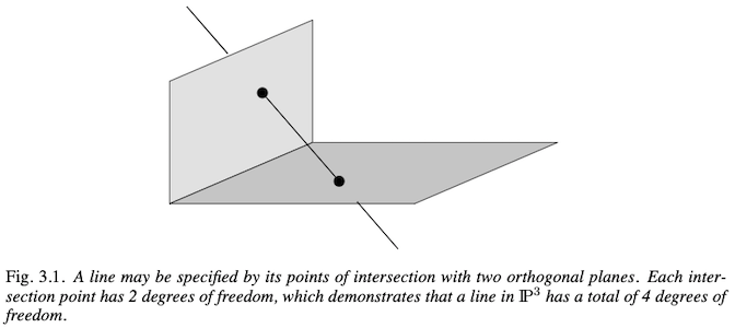
However, to represent a 4 dof would be a homogeneous 5-vector. So there are different representations. Following are three of them:
-
Def. 1: Null-space and span representation (dof: 6)
$$W=\begin{bmatrix}
\mathbf{A}^\top \\
\mathbf{B}^\top
\end{bmatrix}$$$\mathbf{A}$, $\mathbf{B}$ is two points in line.
-
Def. 2: Plucker matrices (dof: 4)
Define by two points:
$$\mathbf{L}=\mathbf{A}\mathbf{B}^\top-\mathbf{B}\mathbf{A}^T$$Define by two planes:
$$\mathbf{L}^*=\mathbf{P}\mathbf{Q}^\top-\mathbf{Q}\mathbf{P}^T$$
$\mathbf{L}^*$ is just the rewrite $\mathbf{L}$:
$$l_{12}:l_{13}:l_{14}:l_{23}:l_{42}:l_{34}=l_{34}^*:l_{42}^*:l_{23}^*:l_{14}^*:l_{13}^*:l_{12}^*$$The plane defined by the join of the point $\mathbf{X}$ and Line $\mathbf{L}$ is:
$$\boldsymbol{\pi}=\mathbf{L}^*\mathbf{X}$$
except $\mathbf{X}$ on line $\mathbf{L}$: $\mathbf{L}^*\mathbf{X}=0$.The point defined by the intersection of the line $L$ and plane $\boldsymbol{\pi}$ is:
$$\mathbf{X}=\mathbf{L}\boldsymbol{\pi}$$
except $\boldsymbol{\pi}$ on line $\mathbf{L}$: $\mathbf{L}\boldsymbol{\pi}=0$. -
Def. 3: Plucker line coordinates (dof: 4)
Only six non-zero element of Plucker matrix:
$$\mathcal{L}={l_{12},l_{13},l_{14},l_{23},l_{42},l_{34}}$$ -
Quadrics and dual quadrics (See p.73)
Estimation - 2D Projective Transformation
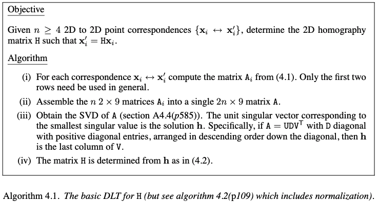
The Direct Linear Transformation (DLT) algorithm
-
Aim to find transformation $H$ given a set of four 2D to 2D point correspondences, $\mathbf{x}_i\leftrightarrow\mathbf{x}_i’$. This gives: $\mathbf{x}_i’=H\mathbf{x}_i$
We can solve $H$ by the cross product: $\mathbf{x}_i’\times H\mathbf{x}_i=0$
Let the $j$-th row of $H$ is denoted by $\mathbf{h}^{1\top}$:
$$H\mathbf{x}_i=\begin{pmatrix}
\mathbf{h}^{1\top}\mathbf{x}_i \\
\mathbf{h}^{2\top}\mathbf{x}_i \\
\mathbf{h}^{3\top}\mathbf{x}_i
\end{pmatrix}$$Let $\mathbf{x}_i’=(x_i’, y_i’, z_i’)^\top$
$$\mathbf{x}_i’\times H\mathbf{x}_i=\begin{pmatrix}
y_i’\mathbf{h}^{3\top}\mathbf{x}_i-z_i’\mathbf{h}^{2\top}\mathbf{x}_i \\
z_i’\mathbf{h}^{1\top}\mathbf{x}_i-x_i’\mathbf{h}^{3\top}\mathbf{x}_i \\
x_i’\mathbf{h}^{2\top}\mathbf{x}_i-y_i’\mathbf{h}^{1\top}\mathbf{x}_i
\end{pmatrix}$$, which could be reformed to:
$$\begin{bmatrix}
\mathbf{0}^\top & -z_i’\mathbf{x}_i^\top & y_i’\mathbf{x}_i^\top \\
z_i’\mathbf{x}_i^\top & \mathbf{0}^\top & -x_i’\mathbf{x}_i^\top \\
-y_i’\mathbf{x}_i^\top & x_i’\mathbf{x}_i^\top & \mathbf{0}^\top
\end{bmatrix}
\begin{pmatrix}
\mathbf{h}^1 \\
\mathbf{h}^2 \\
\mathbf{h}^3
\end{pmatrix}=\mathbf{0}\\
\Leftrightarrow \mathbf{A}_i\mathbf{h}=\mathbf{0}$$, where $\mathbf{A}_i$ is a $3\times9$ matrix and $h$ is a 9D-vector made up of the entries of the of the entries of $H$.
(i) The equation $\mathbf{A}_i\mathbf{h}=\mathbf{0}$ is an linear equation in the unknown $h$.
(ii) $\mathbf{A_i}$ has three rows but only two of them are independent. The third row could be the sum of $x_i’$ times the first row and $y_i’$ times the second.
(iii) We could directly choose $z_i’=1$ for measurement, but other choices are possible.
-
Solving for $H$
Usually we will find multiple point correspondences more than 4. And this leads to over-determined solution. However, due to the measurement noise, the $A$ is not have rand 8. So the target is to minimize $\frac{\lVert\mathbf{A}\mathbf{h}\rVert}{\lVert\mathbf{h}\rVert}$. Which the basic DLT algorithm does:
-
Computational complexity of the SVD to decompose $m\times n$ matrix:
To find U, D, V we need $4m^2n+8mn^2+9n^3$ floating-point operations(flops).
To find only D, V, we need $4mn^2+8n^3$ flops.
-
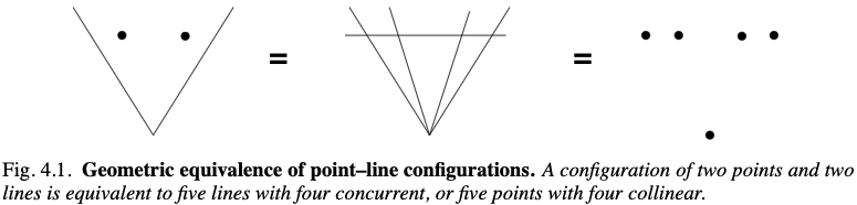
Configuration to determine the homographic transformation:
3 points & 1 line – OK
3 lines & 1 point – OK
2 lines & 2 points – NO
-
Different cost functions
-
Algebraic distance
The DLT algorithm minimizes the norm$\lVert\mathbf{A}\mathbf{h}\rVert$, which is called algebraic distance $\epsilon_i$:
$$d_{alg}(\mathbf{x}_i’,H\mathbf{x}_i)^2=\lVert\epsilon\rVert^2=\lVert\begin{bmatrix}
\mathbf{0}^\top & -z_i’\mathbf{x}_i^\top & y_i’\mathbf{x}_i^\top \\
z_i’\mathbf{x}_i^\top & \mathbf{0}^\top & -x_i’\mathbf{x}_i^\top
\end{bmatrix}\mathbf{h}\rVert^2$$More generally, for two vecotrs $\mathbf{x}_1$ and $\mathbf{x}_2$, the algebraic distance is:
$$d_{alg}(\mathbf{x}_1,\mathbf{x}_2)^2=a_1^2+a_2^2$$
, where $\mathbf{a}=(a_1,a_2,a_3)^\top=\mathbf{x}_1\times \mathbf{x}_2$.
-
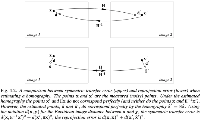
Geometric distance
Notation: $\mathbf{x}$ represent the measured image coordinates; $\hat{\mathbf{x}}$ represent estimated values of the points and $\overline{\mathbf{x}}$ prepresent true values of the points.
The measurement is accurate enough, and the only error is transfer error.
Single image error: $\sum_i d(\mathbf{x}_i’, H\overline{\mathbf{x}}_i)^2$
Symmetric transfer error: $\sum_i d(\mathbf{x}_i’, H\mathbf{x}_i)^2+d(\mathbf{x}_i,H^{-1}\mathbf{x}_i’)^2$
-
Reprojection error - both images
$\sum_i d(\mathbf{x}_i, \hat{\mathbf{x}}_i)^2+d(\mathbf{x}_i’,\hat{\mathbf{x}}_i’)^2$ subject to $\hat{\mathbf{x}}_i’=\hat{H}\hat{\mathbf{x}}_i$
- For affine transformation and below, the DLT algorithm is the same as geometric distance.
-
Sampson error (Skip, ref: p.98)
Statistical cost functions and Maximum Likelihood estimation
Skip. ref: 102
Transformation invariance and normalization
-
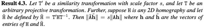
Non-invariance of the DLT algorithm
Suppose we have correspondences $\mathbf{x}_i\leftrightarrow\mathbf{x}_i’$ in image, and we have another transformation $T$ (like origin change, coordinates direction change, etc.). The transformed correspondences will be $\tilde{\mathbf{x}}_i\leftrightarrow\tilde{\mathbf{x}}_i’$, where $\tilde{\mathbf{x}}_i = T\mathbf{x}_i$ and $\tilde{\mathbf{x}}_i’ = T’\mathbf{x}_i’$. Then let $\tilde{H}=T’HT^{-1}$, we will get:
which means:
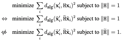
-
Invariance of geometric error
$$d(\tilde{\mathbf{x}}_i’, \tilde{H}\tilde{\mathbf{x}})=d(T’\mathbf{x}‘, T’HT^{-1}T\mathbf{x})=d(T’\mathbf{x}‘, T’H\mathbf{x})=d(\mathbf{x}’,H\mathbf{x})$$
-
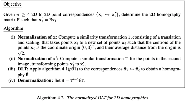
Normalizing transformations
Iterative minimization & Robust estimation (RANSAC)
skip (ref: 110)